Example 1 - Two-phase bar
A bar that consists of a stiffer and a softer material with Youngs’s moduli \(E_{1}\), and \(E_{2}\). The bar is fixed on the left side and a displacement \(u\) is applied to the right side. The configurational forces on the interface should be computed using the Abaqus plug-in.

Theory
Kollnig et. al. [1] provide a theoretical solution for the configurational forces on the interface. The solution can be computed symbolically using sympy. First, define symbolic and real quantities. The Poisson’s ratio \(\nu\) is set to zero.
>>> import sympy as sy
>>> (
...     E1,  # youngs modulus of left side
...     E2,  # youngs modulus of right side
...     A,  # cross-section of beam
...     l,  # total length of beam
...     l1,  # length of left side
...     e,  # total strain
...     e1,  # strain of left side
...     e2  # strain of right side
... ) = sy.symbols("E1 E2 A l l1 e e1 e2", real=True)
>>> E1_val = 210_000  # MPa
>>> E2_val = E1_val / 2  # MPa
>>> l1_val = 10  # mm
>>> l_val = 2 * l1_val
>>> A_val = 10  # mm^2
>>> u_val = 0.1  # mm
Next, the energy of the beam is formulated as
>>> ALLSE = 0.5 * E1 * e1**2 * A * l1 + 0.5 * E2 * e2**2 * A * (l - l1)
The strain \(e = \frac{u}{l} = e_{1} + e_{2}\) is the sum of the strain e1 in the left material and the strain e2 in the right material. This kinematic relationship between e1, e2 and e is used to eliminated e2.
>>> e2_expr = sy.solve(sy.Eq(l*e, l1*e1 + (l - l1) * e2), e2)[0]
>>> ALLSE = ALLSE.replace(e2, e2_expr)
>>> e2_expr
(e*l - e1*l1)/(l - l1)
Furthermore, minimizing the strain energy ALLSE leads to the quasi-static solution of e1. For this reason, the derivative of ALLSE with respect to the not constrained strain e1 is set to zero. Consequently, e1 is eliminated.
>>> e1_expr = sy.solve(sy.Eq(0, ALLSE.diff(e1)), e1)[0]
>>> ALLSE = ALLSE.replace(e1, e1_expr)
>>> e1_expr
E2*e*l/(E1*l - E1*l1 + E2*l1)
Finally, the total derivative of the strain energy with respect to the position of the interface is computed. The symbolic values are replaced by the numeric values. This results in the expected configurational force in x-direction at the interface.
>>> dAllSE_dl1 = ALLSE.diff(l1)
>>> cfx_at_interface_theory = dAllSE_dl1.xreplace({
...     A: A_val,
...     E1: E1_val,
...     E2: E2_val,
...     e: u_val / l_val,
...     l: l_val,
...     l1: l1_val
... })
>>> cfx_at_interface_theory  # N
11.6666666666667
Using the Abaqus plug-in
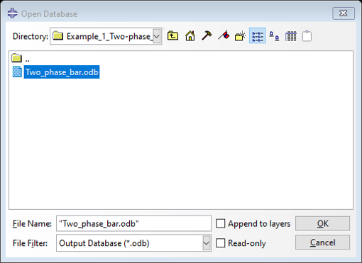
This section describes how to compute the configurational forces using the Abaqus plug-in. First, simulate the *.inp file using the Abaqus solver to obtain the *.odb. Open the *.odb in Abaqus CAE. Make sure that the file is not opened Read-only.
Navigate to Plug-ins -> Conf. Force
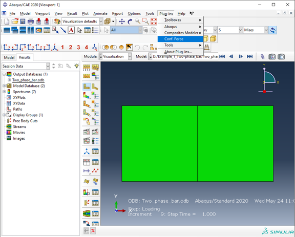
The plug-in GUI opens.
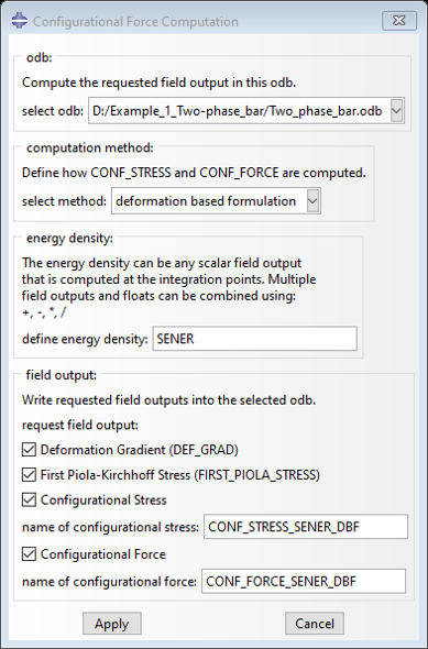
The odb drop-down lists all open odb files.
Configurational stresses and forces can be computed using various methods. Select your desired method.
Configurational stresses and forces need a energy density. Set the energy density to SENER to only consider the elastic strain energy density. Or use SENER+PENER to build the sum of elastic and plastic energy density.
Select quantities in the field output section that are computed and saved into the odb.
The name of the configurational stress and force can be modified to compute them with varying energy desnsities.
Click Apply to start the computation.
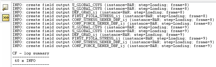
After all requested quantities are written into the odb, a log summary is printed.
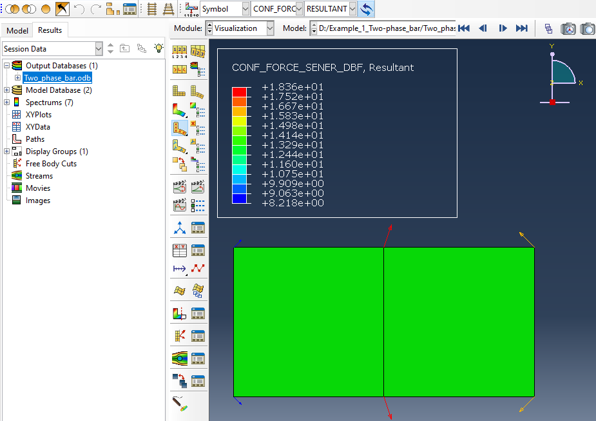
The requested field outputs of ConForce can be selected and plotted as vector plot.
Verify Results
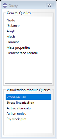
For the comparison with the theoretical values, the x-component of the configurational forces on the interface are summed up. This can be done by probing values in Abaqus. Navigate to Tools -> Query -> Prove values.
Select Node as Probe position and activate the x-component of the configurational forces in the viewport. Select the two nodes on the interface in the viewport.
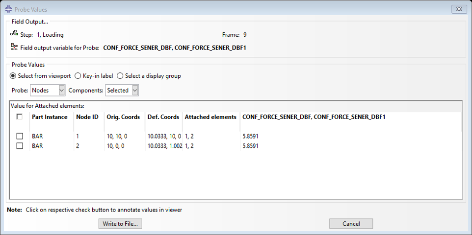
The plugin computes configurational forces of
>>> cfx_at_interface_plugin = 5.8591 + 5.8591  # N
>>> cfx_at_interface_plugin
11.7182
The theoretical and computed values differ by a factor of
>>> cfx_at_interface_plugin / cfx_at_interface_theory
1.00441714285714